Occupational Soundscapes – Part 15: Community Noise

     The discussions of occupational soundscapes throughout this series have implied a certain perspective, either that of one exposed to noise or that of one responsible for its management and control.  In some cases, both perspectives are taken simultaneously.  Other perspectives are also possible, however.
     For anyone not engaged in the activities that generate noise of concern, the nature of a soundscape changes.  As an example, consider a professional auto race or outdoor concert.  Direct participants (e.g. racers, performers) experience occupational noise exposure, as do support personnel (e.g. course marshals, sound technicians, security).  Spectators are exposed to recreational noise; that is, the exposure is optional.
     Sound that escapes the event venue to the surrounding area becomes community noise.  The same is true of commercial and industrial facilities, where continuous operation can cause greater impacts on nearby communities than discrete events.

     Commercial and industrial facilities are among several contributors to community noise.  It also consists of recreational (e.g. music, sporting events) and transportation (e.g. aircraft, rail, and highway traffic) sources.  Agricultural, mining, and construction activities also contribute to community noise.
     In this installment of the series, community noise is treated as an extension of an occupational soundscape, specifically, a commercial or industrial noise source.  Other types of noise sources are considered only to the extent to which they are in the purview of the commercial or industrial site and its management.
     To clarify terms in use, consider the distinction between commercial and industrial sites.  Commercial sites include retail outlets, office buildings, financial institutions, and other typically “quiet” businesses.  Industrial sites include manufacturing plants, warehouses, distribution centers, and other storage areas.  This distinction is relevant to property zoning, but is less valuable to the current discussion; unless the context makes the distinction necessary, these terms may be used interchangeably.
     It is plausible that an industrial noise source interferes with nearby commercial operations, for example.  Likewise, healthcare, educational, recreational, and agricultural areas may also be impacted.  However, the primary concern of this presentation is the effect of industrial noise on residential areas.  A residential area can include various types of domiciles, including single- and multi-family dwellings, seasonal residences, and mobile homes.
     Residential areas are the primary concern of community noise because of the quality-of-life issues that it can cause, including interference with sleep.  The sanctity of one’s home is more likely to be upheld, whether in public opinion or legal proceedings, than almost any other concern that may be raised.  It is the basis for many noise ordinances, though their scope tends to include all sources of community noise.  At many sites, residential areas expand and encroach upon industrial facilities.  Pre-existing residential development is rarely helpful in defending an industrial noise source against a nuisance complaint.
     In the absence of sufficient regulation or enforcement, activists may emerge.  To avoid negative publicity and its snowballing effects, many organizations strive to maintain “good neighbor” status with surrounding communities.  This may include implementing measures to reduce noise below required levels.  This approach may preclude vigorous opposition to continued operations or expansion plans.  Once community support falters, the breadth of opposition tends to expand to other issues; maintaining a collaborative relationship with vocal advocates is an advisable strategy.

Community Noise Control
     Much of the information presented in the subseries on noise control (Parts 11 – 14) is also applicable to community noise, albeit with slight modification.  In this section, some modifications, or extensions, of the noise control presentation relevant to community noise are addressed.

Noise Control Planning (see Part 11)
     Creating a sound survey map, or noise contour map, of the entire site (e.g. facility exterior) simplifies understanding of the magnitude of noise concerns and, thus, prioritization of remediation projects.  All natural and constructed features of the property, including building structures, should be included on the map.  The nature of the surrounding areas and their boundaries should also be clearly labeled.  An example site sound map is shown in Exhibit 1.  The example is quite generic; a legend of sound levels and other information are needed for application to a real-world noise control effort.

     Details should be added to a sound survey map selectively; too much information or poor formatting can clutter a map, diminishing its utility.  Useful information may include peak and average sound levels, duration and frequency of peak levels, and relevant temporal data (e.g. time of day or year).  Methods of quantifying sound levels are discussed further in the section on noise measurement, below.

Hierarchy of Controls (see Part 11)
     The hierarchy of controls remains valid, with one exception:  PPE is not available as a last-resort protection from community noise.  Well-informed neighbors may choose to utilize HPDs to mitigate their exposure or annoyance, but they cannot be compelled to do so.  Community noise must be controlled at higher levels of the hierarchy, with elimination of the source remaining the most desirable solution.

The SPR/ETI/PAP Model (see Part 11)
     The source-path-receiver (SPR) model continues to be “the” approach to noise control.  The receiver portion of the model, however, must be deemphasized in the community noise context even more than it is for occupational noise.  Few receiver-protection options exist and their effects are minimal, reinforcing the priority of controlling noise at its source.

Source Noise Control (see Part 12)
     Significant sources of community noise include many that are often easily overlooked when conducting an occupational noise survey.  Activities that take place, and equipment that operates, on the exterior of a facility are often unnoticeable to the vast majority of workers inside.  It is precisely these noise sources, however, that are often most noticeable in surrounding areas.  The facility often provides little or no attenuation of these sounds; worse, the structure may reflect sound, exacerbating the situation.
     Outdoor equipment that contributes to community noise includes air handlers and exhaust fans, air compressors, generators, pumps and pipelines, public address (PA) systems, and much more.  Facilities with equipment operating around the clock face additional challenges; generally quieter periods of the day (e.g. nighttime) usually require lower levels of sound emission.
     Part 12:  Source Noise Control contains information that can be applied to much of this equipment.  For example, the “Hydraulic Noise” section can be applied to outdoor pipelines as well as indoor fluid-handling systems.  Helpful information on fans is provided in the “Aerodynamic Noise” section; Exhibit 2 depicts an example of how a minor change in equipment specification can have a profound impact on community noise.

     Exhibit 3 depicts another type of aerodynamic noise issue, one of noise generated without engaging in any particular activity.  In this example, noise is generated by a passive interaction with the environment.  Wind passing a smoke stack generates noise, such as a whistling sound; attaching a spiral with varying pitch modifies the airflow sufficiently to prevent noise.  Similar phenomena may be experienced with antennae, flag poles, or cables used to stabilize similar structures (i.e. guy wires); a similar solution can be implemented in each case.
     Delivery vehicles can cause significant disturbance, particularly at a high-throughput facility, such as a distribution center (DC).  In addition to 18-wheelers, box vans, or other types of vehicle that may arrive and depart a site regularly, there is often a fleet of logistics and material-handling vehicles (e.g. “yard dogs,” forklifts) that operate continuously on the premises.  Operators of these vehicle are typically evaluated for speed and accuracy, while the noise generated by their activities goes unnoticed.  Unnoticed, that is, by those within the facility; nearby residents may have a very different experience.  Vehicle and equipment maintenance, in conjunction with awareness and “quiet operation” training, are essential tools for minimizing this type of community noise contribution.
     Given the array of activities and facility and equipment variations that exists, noise sources not considered here certainly exist.  An evaluation must be broad to ensure that all noise sources for which an organization is responsible – directly or indirectly – are identified and proper controls activated.

Path Noise Control (see Part 13)
     An industrial facility is typically treated as a single source in community noise discussions, though several discrete sources may exist within it.  Facilities are typically on large plots of land, placing potential receivers of noise at significant distances from the source.  At these distances, individual noise sources are often indistinguishable, as the spectral components of each coalesce into a single perceived broadband noise.  In noise control terms, the surrounding areas are in far field, usually free field, conditions.
     Directionality of noises must be factored in to community noise analyses.  Outdoor equipment operating near the main structure of a facility exhibits increased directivity (e.g. Q = 4; DI = 6 dB).  If placed among multiple structures, directivity can increase further (e.g. Q = 8; DI = 9 dB).  Noise emanating from inside a facility can also exhibit directionality when doors are left open, for example.  Such effects are more difficult to predict; multiple scenarios should be represented in sound surveys to ensure adequate controls are developed.
     Barriers erected along property boundaries are common responses to community noise concerns.  A conspicuous example of this approach is the evermore-ubiquitous walls lining interstate highways.  While reducing the exposure of frontage properties, reverberant canyons are created, within which noise exposures and associated risks increase.  Fortunately, the scale of typical industrial sites tend to make problematic reverberant fields much less common.
     In addition to air-borne sound transmission, ground vibrations can also transmit unwanted energy to surrounding areas.  This is typically low-frequency noise caused by mining activities, heavy equipment operation, manufacturing with very large stamping presses, or similar operations.  The potential for this type of transmission is influenced by the geological composition of the site, construction techniques, and process parameters.  It must be considered carefully, as it may require a “financial solution;” a viable technical solution may not exist.

Receiver Noise Control (see Part 14)
     As mentioned above, it is unreasonable, not to mention unlawful, to expect the community-at-large to accept the use of HPDs in “everyday life” as appropriate.  Other options for receiver noise control are scarce and of limited utility.
     Activities can be scheduled for times of day – or year – that they will be least disruptive; maximum sound levels still apply.  This option is only feasible for infrequent or nonroutine activities, such as some construction or maintenance tasks.  Noise generated by frequent or continuous activities, or at high intensity, must be managed with more-sophisticated controls.

Effects of Community Noise
     The effects of occupational noise exposure, presented in Part 8, can also be caused by community noise.  However, community noise is typically experienced at lower intensity, while engaged in activities unrelated to the noise source.  A change in circumstances can have a profound effect on the perception and acceptability of sound; the experience of exposure is drastically changed.
     The types of activities typically discussed in the context of community noise reflects the emphasis on protecting residential areas from intrusive noise.  The most-prominent topic is interference with speech communication; the concepts presented in Part 9, such as masking and intelligibility, are relevant to both community and occupational noise exposures.  The change in setting, however, eliminates the use of a limited, standard vocabulary or sophisticated electronic communication system as viable solutions.
     Community noise can impact various types of speech communication, including casual conversation, professional interactions (e.g. legal or medical consultation), educational lectures, and commercial transactions (e.g. sales presentation or contract review).  The lack of visual cues available during telephone conversations and modifications of speech that occur during reproduction and transmission increase susceptibility to interference.  Similarly, TV and radio broadcasts and other forms of audio presentation of speech are subject to the same limitations.
     While the speech intelligibility concern may be reduced or eliminated when listening to music, the enjoyment of music can be degraded by the infiltration of community noise.  Playing music, or engaging in any activity that requires concentration, can be negatively impacted by unrelated noise.  The consequences of poor performance on these tasks must be considered.  A student’s inability to concentrate on homework leads to low grades; a misbalanced checkbook leads to overdrafts, missed payments, fees, or other complications.  Superficial reading of an insurance policy, mortgage refinancing agreement, or other legal document has far-reaching consequences; an incorrectly wired electrical outlet leads to shock or fire.  The dangers of distraction, spanning all potential activities of a population, are innumerable.
     Periods of relaxation and sleep are highly influential on quality-of-life assessments.  Relaxation activities include some of those mentioned above; many activities typically associated with “quiet” may also be included, such as reading, journaling, painting, meditation, yoga, nature walks, and others.  Soaking up the sun while sipping a mai tai is the quintessential relaxation activity.  Excessive noise is disturbing and can render true relaxation unattainable.
     When noise disturbances extend into periods reserved for sleep, consequences escalate rapidly.  Interference with other activities causes annoyance, but frequent sleep disturbance can result in serious health issues.  Even when a person becomes accustomed to noise, levels of stress hormones increase and sleep is less restorative.  Noise exposure causes increases in heart rate and blood pressure (BP), counteracting the usual drop in BP one experiences during sleep.  The combination of normal physiological responses to noise can result in cardiovascular disease and has been linked to increased rates of diabetes.
     These long-term effects, like noise-induced hearing loss (NIHL), are not obvious right away.  However, frequent symptoms of sleep deprivation, such as fatigue or lethargy, difficulty concentrating, or irritability may be warning signs that a serious chronic problem exists or could develop without appropriate interventions.
     Prolonged, unmitigated noise that causes any of the above impacts to those in the vicinity of a source facility is likely to degrade the operating organization’s standing in the community.  Declines in public opinion of the facility operator are commensurate with the duration or severity of the nuisance it creates.  The frequency of corresponding complaints, legal and political actions, and public outcries are likewise correlated.
     Though industrial noise has been shown in a number of studies to be a lesser problem than transportation noise, a fixed site provides a single, identifiable target for backlash.  Assigning culpability for highway traffic noise, for example, is not so simple; addressing it requires action by various agencies and political figures at multiple levels of government.  When the nuisance is created by aircraft, or airport operations, the difficulty is magnified many-fold, as it must involve the federal government in addition to all other entities.  For these reasons, industrial sites may have to endure greater scrutiny than their “offenses” warrant until scientific exoneration redirects attention to its rightful recipients.

Quantifying Community Noise – Measurement
     When citing community noise levels, exactly what noise has been measured must be specified, lest the values be misleading or confusing.  An ambient noise measurement accounts for all sources, including the source of interest, all forms of transportation, all other activities, and natural sounds, such as birdsong or rustling of leaves.  Specific noise is that attributed to the source under scrutiny and residual noise is that which remains when the specific noise is absent.
            Stated another way, specific noise – the noise of concern – is the difference between ambient noise and residual noise.  A specific noise may be defined by measuring the ambient and the residual, using “Sound Math” (Part 4):
     Ambient Noise  =  Residual Noise  +  Specific Noise.
     The term “background noise” may be used to refer to the level of sound when a specific noise is not audible, though it may be present; it could also refer to an exposure index, such as L90 (see Part 6).  The use of terms varies by author; readers are cautioned to verify definitions when consulting multiple sources.  The definitions provided above are deemed to be least ambiguous; the terms are used in this manner throughout this presentation.
     Community noise is typically defined in terms of equivalent continuous sound levels (see Part 6).  Several can be cited, including:

• Ld – daytime equivalent continuous sound level (dBA); the average sound level during the period from 07:00 to 22:00 (7 AM to 10 PM).
• Ln – nighttime equivalent continuous sound level (dBA); the average sound level during the period from 22:00 to 07:00 (10 PM to 7 AM).
• Ldn – day-night average sound level, or DNL (dBA); the average sound level during a 24-hr period.  A 10-dBA penalty is applied to nighttime values to reflect the increased intrusiveness of noise at night:

DNL is often the first, sometimes the only, community noise metric cited when assessing acceptability of, for example, development or expansion plans.
In the absence of a dominant noise source, such as an industrial site, highway, or airport, an estimate of DNL, based on population, can be calculated:  Ldn = 23 + 10 log (PD) (dBA), where PD is the population density (people/sq km) of the area; this estimate can be used where PD > 200 people/sq km.

• Le – evening equivalent continuous sound level (dBA); the average sound level during the period from 19:00 to 22:00 (7 PM to 10 PM).  When Le is used, the definition of daytime hours, for calculation of Ld, is changed to the period from 07:00 to 19:00 (7 AM to 7 PM).
  
• Lden – community noise equivalent level, or CNEL (dBA); the average sound level during a 24-hr period.  A 5-dBA penalty is applied to evening values (“relaxation time”) and a 10-dBA penalty is applied to nighttime values (“sleep time”):

• Normalized Ldn is derived by applying correction factors to measured Ldn values.  Descriptions of corrections and the magnitude of each are given in Exhibit 4.  The corrections cited were originally established to correlate actual community response in various circumstances to anticipated rates of complaints, “community action,” etc.  Increments of 5 dB are used, as the original authors deemed this to be the limit of accuracy.  An additional +12 dB correction is included in ANSI S12.9 for “highly impulsive sounds,” such as gunfire, jack-hammering, pile-driving, or riveting.
  

• Rating level (Lr) is similar to normalized Ldn; penalties are assessed to adjust an A-weighted continuous equivalent sound level to quantify the annoyance caused by a sound.  It takes the form Lr = LAeq + KI + KT + KR + KS, where KI is an impulse penalty, KT is a tonality penalty, KR is a time-of-day penalty, and KS is a “source and situation” penalty.

The procedure for determining a rating level is defined by international standard (ISO 1996), but the penalties vary by national jurisdiction.  Readers interested in the rating level method should consult the ISO standard and local regulations.

     When conducting a sound survey, several variables must be considered; documenting conditions in which measurements are taken is critical to understanding the results.  It should be obvious that modification of source parameters can impact measurements significantly.  These include equipment operating at reduced vs. full capacity, a facility that is partially vs. fully staffed, and any other circumstances that affect sound generation or activity levels.
     Placement of measurement equipment must also be carefully considered to ensure valid data are obtained.  Microphones are typically placed 1.2 – 1.8 m above the ground, unless topography dictates otherwise (e.g. line of sight to source lost).  Measurements should not be taken over paved areas or near large objects, such as buildings, unless the objective is to document the effects these features have on measurements.  To avoid excessive influence on measurements, microphones should be placed at least 7.5 m (19 m recommended) from large reflective surfaces and at least 1.5 m from small objects (e.g. trees, poles, etc.)  Even the presence of a person near a sound meter can affect measurements; remote monitoring options should be considered whenever possible.
     Seasonal variation in measurements can be caused by changes in plant growth (e.g. tree canopy) and insect and wildlife activity (e.g. buzzing swarms, honking flocks of geese, croaking frogs, etc.)  Meteorological conditions fluctuate more rapidly, potentially causing significant variation in sound measurements.  The influence of these fluctuations is explored further in the “Calculation” section below.
     It is common practice to begin a sound survey in locations that exhibit high potential for complaints, such as boundaries between the source site and residential areas.  Identifying these locations on a site map with additional notes describing factors that influence measurements provides a rapid reference that is useful throughout a noise investigation and beyond.
     It may be necessary to repeat measurements at times when different conditions exist, or conduct long-term monitoring, to capture as much of the variability as possible.  Doing so facilitates identification of the worst case, which may be that the solution chosen under one set of conditions exacerbates a noise concern under another.  Without thorough documentation of measurement conditions, sound level values recorded contain little insight; identifying and resolving this type of issue becomes impossible.

     Other measures of sound exposure, such as noise dose (see Part 6), loudness and noisiness (see Part 7), and speech intelligibility (see Part 9) remain valid for community noise exposure.  However, it is more common to apply these concepts to individuals; as such, these measures may only enter a discussion of community noise as support for a nuisance complaint that has escalated to legal action where professional analysts are employed to investigate the validity of claims or potential resolutions.
     One collective metric that can be used to assess community noise is the total weighted population (TWP) effected.  TWP uses weighting factors associated with DNL ranges to assess the magnitude of annoyance caused by a noise source.  It is calculated as follows:  TWP = ∑i (Wi x Pi), where Wi is the weighting factor for a specific range of DNL, tabulated in Exhibit 5, and Pi is the number of people subjected to DNLs in that range.

     To compare the community impact of disparate noise sources, a noise impact index (NII) can be calculated for each:  NII = TWP/∑i Pi, where TWP and Pi are defined above.  Either TWP or NII could be used to prioritize allocation of limited resources needed to pursue noise reduction initiatives.

Quantifying Community Noise – Calculation
     Predictive calculations of sound levels can be performed in the planning phase of a greenfield or brownfield development, expansion project, or other change in operations that are anticipated to significantly affect the community soundscape.  A series of calculations is needed to account for all relevant variables.  Fortunately, each computation is fairly simple, though the number of variables and look-up tables involved may seem daunting at first glance.  The configuration of calculations varies slightly among reference sources; the form presented here attempts to simplify the progression where possible.
     Anticipated sound level at any receiver location is calculated, per octave band, as follows:  Lp = Lw – Atotal (dB), where Lp is the SPL at the defined location (dB), Lw is the source PWL (dB), and Atotal is the total attenuation (dB).
     Total attenuation accounts for environmental factors that influence sound propagation, as well as existing noise control measures:  Atotal = Adiv + Aair + Aenv + Amisc, where Adiv is attenuation resulting from geometrical divergence, Aair is air absorption, Aenv is attenuation due to environmental effects, and Amisc is attenuation attributed to all other causes.
     Geometrical divergence reduces sound levels according to the inverse square law (see Part 3); this attenuation is calculated as Adiv = 20 log (r) + C (dB), where r is the distance between source and receiver and C = 10.9 when r is measured in meters (C = 0.6 when r is measured in feet; however, use of metric dimensions is advised to maintain consistency with remaining calculations).
     Air absorption, or atmospheric attenuation, depends, in order of decreasing influence, on relative humidity, frequency, and temperature.  This attenuation is calculated as Aair = α’ r/1000 (dB), where α’ is the air attenuation coefficient (dB/km) at standard pressure (1 atm).  Values of α’ are tabulated in Exhibit 6; coefficients corresponding to intermediate parameter values can be found by interpolation.

     Environmental attenuation effects include the influences of ground effects, wind speed and direction, and temperature gradients.  Attenuation due to ground effects is determined by one of two methods, depending on whether propagation is short- or long-range.  Both methods require identification of ground conditions between source and receiver as hard, soft, very soft, or mixed.
     Hard ground includes concrete, asphalt, highly-compacted or tamped soil, bodies of water, and other low-porosity, highly-reflective surfaces.  Soft ground includes areas covered with grass, shrubs, or other vegetation, and porous ground suitable for such growth.  Very soft ground includes fresh snow (i.e. not compacted), ground covered in pine needles or other loose material, and water-saturated soil.  Mixed ground has areas of both hard and soft ground between source and receiver.

     Short-range propagation is defined as that up to 100 meters (r < 100 m); the diagram in Exhibit 7 depicts the direct and reflected sound propagation paths between source and receiver.  To determine short-range attenuation, locate the section of Exhibit 8 for the ground condition present, then, within it, the attenuation value(s) corresponding to source and receiver parameters.  At angles of incidence greater than 20°, reflection from soft ground increases such that it can be treated as hard ground.   Attenuation of mixed ground is determined by interpolation between the hard and soft ground values according to the proportion of each.  Negative attenuation values indicate that reflections increase sound levels at the receiver.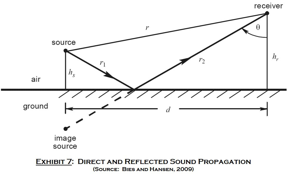

     To determine ground-effect attenuation for long-range propagation (r > 100 m), there are three zones between source and receiver to be considered, as shown in Exhibit 9.  The source zone length is 30 times the source height (hs) and the receiver zone length is 30 times the receiver height (hr), each with a maximum of r, the source-to-receiver distance.  When 30 hs + 30 hr > r, a middle zone lies between.
     Each zone is assigned a ground factor, G, based on the ground conditions in that zone.  For hard ground, G = 0, for soft ground, G = 1, and for mixed ground, G is equal to the proportion of the zone consisting of soft ground.  For very soft ground, G = 1 can be used, though attenuation values will be underestimated, particularly in the lowest frequencies.
     Long-range ground-effect attenuation (Agr) is the sum of attenuations in the three zones (two, if no middle zone exists):  Agr = As + Ar + Am.  Zone attenuations are found using Exhibit 10; factors a, b, c, and d, used to calculate source and receiver zone attenuations, are tabulated in the lower section.  To calculate middle zone attenuation, use factor e = 1 – [30 (hs + hr)/r].

     Attenuation due to wind and temperature gradients are difficult to predict precisely.  Nonetheless, it is useful to have a general understanding of the effects varying conditions can cause.
     Sound propagation is affected by air temperature.  Normal daytime conditions include a negative temperature gradient (temperature drops with altitude), or a “lapse,” creating a shadow zone at ground level, as depicted in Exhibit 11A.  Sound levels in the shadow zone can be 10 – 20 dB lower than predicted by ground-effect attenuation.
     At night, normal conditions include a temperature “inversion,” or positive temperature gradient, causing sound to be projected toward the ground.  In this condition, depicted in Exhibit 11B, environmental factors provide little to no attenuation at distances up to several hundred meters; attenuation may even become negative.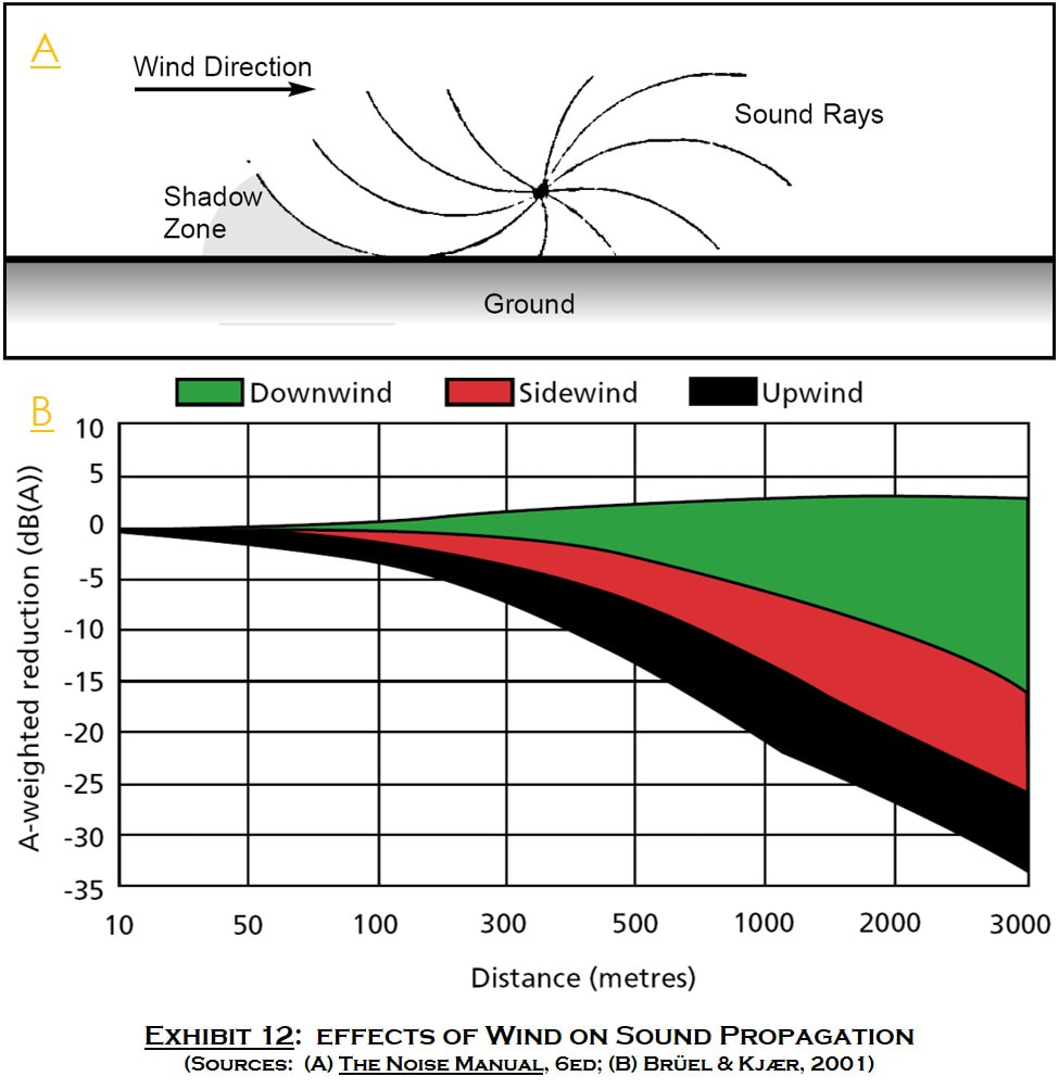

     Wind creates similarly dichotomous attenuation effects.  Upwind of a source, a shadow zone is created, as shown in Exhibit 12A.  Downwind of a source, sound can be intensified; the degree depends largely on wind speed.  Exhibit 12B charts potential broadband sound level changes for each of these conditions, as well as in crosswind.
     As these effects demonstrate, it is important to document the conditions under which measurements are taken or are assumed in calculations.  Downwind measurements are usually preferred to capture “worst-case” conditions.  However, prevailing conditions and locations of interest may require upwind measurement.  Again, documentation of conditions is necessary to compare results of multiple measurements and glean needed insight from recorded data.

     Miscellaneous effects include attenuation due to barriers, foliage (trees and bushes), meteorological conditions, and any other feature that previous calculations have not captured.  Attenuation attributed to barriers can be determined as discussed in Part 13, though their effectiveness at large distances is low.
     Foliage is not the attenuator that many seem to think it is; up to 100 m of dense forest is needed to provide significant broadband sound level reductions.  The table in Exhibit 13 provides octave-band attenuation rates for foliage.  Each component of Amisc may be small, but should be included in total attenuation.

     Attenuation due to precipitation and fog is negligible, but it may affect measurements in other ways.  Heavy rain, for instance, can raise the residual noise level and could potentially infiltrate microphones or equipment circuitry, creating errant data or instrument damage.

     Once Lp is calculated for each octave band, the values can be logarithmically added to obtain a broadband SPL.  Frequency weighting can also be applied to obtain an A-weighted broadband sound level (dBA).  A directivity correction can be applied to the broadband level if directionality has not been captured in spectral calculations.  An intermittency correction can also be applied, using an appropriate exchange rate (see Part 6).  An impulsivity adjustment can also be made (see Part 6) if impulsive sounds comprise a significant portion of exposure.

Standards and Regulations
     A number of organizations, across the globe, publish standards related to various noise issues, including measurement of community noise.  Among them are ISO, ANSI, US EPA, OSHA, and many other regulatory bodies and professional organizations.  Though many of these standards tend to converge over time, a thorough review is implausible.
     The good news is that all of the standards need not be known.  Determining which organizations promulgate standards relevant to a specific locale focuses initial research.  Later, research can be expanded to seek additional information, best practices, or alternative explanations that aid implementation of needed noise control measures.
     The regulatory landscape is even more difficult to navigate.  Every jurisdiction defines its own requirements; a single location could be subject to regulations established by multiple levels of government.  There is no guarantee that requirements will be consistent or compatible.  Worse, the order of preemption may be unclear.
     This portrayal is intended not to discourage, but to prepare readers for potential challenges.  To this end, a very basic guideline is offered:

• Research statutes and regulations published by each jurisdiction (e.g. level of government) in which the subject facility and surrounding area is located.  If the affected area crosses jurisdictional boundaries, repeat the process for each jurisdiction.
• Research preemption laws in each jurisdiction to establish priority of conflicting requirements.
• When searching for relevant requirements, include “zoning” and other relevant keywords, in addition to “noise,” to discover useful information that might be easily overlooked.
• If strict guidance (e.g. regulation or statute) has not been established for a site’s jurisdiction, create a standard based on nearby jurisdictions and relevant guidelines and recommendations.
• To the extent possible, internally standardize practices and requirements when operating multiple facilities.
• Consult the EPA’s “Model Community Noise Control Ordinance” or similar regulatory outline to predict potential future requirements.
• If no other guidance is available, pursue the EPA-recommended 55-dBA DNL for residential areas; this is the value deemed protective of community well-being with an “adequate margin of safety.”  Slightly higher DNL may be acceptable for nonresidential areas.
• Conduct the most-thorough sound survey possible; better data yield better results.
• Proactively engage with regulators and community representatives to prevent contentious situations and maintain good standing.
• Pursue continuous improvement in all areas, including measurement, noise control, and community engagement.

     For additional guidance or assistance with Safety, Health, and Environmental (SHE) issues, or other Operations challenges, feel free to leave a comment, contact JayWink Solutions, or schedule an appointment.

     For a directory of “Occupational Soundscapes” volumes on “The Third Degree,” see Part 1: An Introduction to Noise-Induced Hearing Loss (26Jul2023).

References
[Link] The Effects of Noise on Man.  Karl D. Kryter.  Academic Press; 1970.
[Link] “Information On Levels Of Environmental Noise Requisite To Protect Public Health and Welfare With An Adequate Margin Of Safety.”  The U.S. Environmental Protection Agency Office of Noise Abatement and Control; March 1974.
[Link] “Model Community Noise Control Ordinance.”  U.S. Environmental Protection Agency; September 1975.
[Link] Noise Control in Industry – A Practical Guide.  Nicholas P. Cheremisinoff.  Noyes Publications; 1996.
[Link] Environmental Noise.  Brüel & Kjær; 2001.
[Link] “Noise and Vibration.”  Evan Davies in Plant Engineer’s Reference Book, 2ed.  Dennis A. Snow, ed.  Reed Educational and Professional Publishing Ltd.; 2002.
[Link] “Noise – Measurement And Its Effects.”  Student Manual, Occupational Hygiene Training Association; January 2009.
[Link] Engineering Noise Control – Theory and Practice, 4ed.  David A. Bies and Colin H. Hansen.  Taylor & Francis; 2009.
[Link] “Environmental Noise Pollution in the United States: Developing an Effective Public Health Response.”  Monica S. Hammer, Tracy K. Swinburn, and Richard L. Neitzel.  Environmental Health Perspectives; February 2014.
[Link] “Review of 60 U.S. Environmental Community Noise Ordinances.”  John Eichwald, Padmaja Vempaty, and Yulia Carroll.  The Hearing Journal; July 2021.
[Link] The Noise Manual, 6ed.  D.K. Meinke, E.H. Berger, R.L. Neitzel, D.P. Driscoll, and K. Bright, eds.  The American Industrial Hygiene Association (AIHA); 2022.
[Link] “Technical Guide for:  Noise Control – Engineering Controls, Work Practices, & Administrative Controls.”  Georgia Tech; May 2023.
[Link] 40 CFR Part 211 – Product Noise Labeling. EPA.
[Link] US Code Title 42:  The Public Health and Welfare; Chapter 65 – Noise Control.
[Link] US Code Title 42:  The Public Health and Welfare; Chapter 85, Subchapter IV – Noise Pollution
 
Jody W. Phelps, MSc, PMP®, MBA
Principal Consultant
JayWink Solutions, LLC
[email protected]